Tutorial
If you have already installed srim then lets get started! If not please make sure to look at installation first.
In this tutorial we will cover all of the basics of pysrim.
- running a TRIM simple calculation
- analyzing TRIM calculation output files
Most emphasis will be put on what is possible for analysis of SRIM calculations. Since all output files will be exposed as numpy arrays the sky is the limit for plotting.
We will assume python 3 for this notebook and you should be using it too. Python 2.7 is going be depreciated in 2020.
import os

import numpy as np
import matplotlib.pyplot as plt

from srim import TRIM, Ion, Layer, Target
from srim.output import Results
There are not too many important objects to import from srim. The first srim import is for all of the components needed for automating a SRIM calculation. While the second import is for the output results.
Run a SRIM Calculation
Running a srim calculation is much like the gui that SRIM provides.
Concepts:
- a list of Layers forms a Target
- a Layer is a dict of elements, with density, and a width
- an Element can be specified by symbol, atomic number, or name, with a custom mass [amu]
- an Ion is like an Element except that it also requires an energy in [eV]
# Construct a 3MeV Nickel ion
ion = Ion('Ni', energy=3.0e6)

# Construct a layer of nick 20um thick with a displacement energy of 30 eV
layer = Layer({
        'Ni': {
            'stoich': 1.0,
            'E_d': 30.0,
            'lattice': 0.0,
            'surface': 3.0
        }}, density=8.9, width=20000.0)

# Construct a target of a single layer of Nickel
target = Target([layer])

# Initialize a TRIM calculation with given target and ion for 25 ions, quick calculation
trim = TRIM(target, ion, number_ions=25, calculation=1)

# Specify the directory of SRIM.exe
# For windows users the path will include C://...
srim_executable_directory = '/tmp/srim'

# takes about 10 seconds on my laptop
results = trim.run(srim_executable_directory)
# If all went successfull you should have seen a TRIM window popup and run 25 ions!
The following code does a quick SRIM calculation of a 3 MeV Nickel ion
in a nickel target. We have set the displacement energy for Nickel at
30 eV with a density of 8.9 [g/cm^3]. Also notice that after running
the simulation with trim.run the results are automatically parsed
for us. After the calculation has completed many times we will want to
copy the results to a different directory.
output_directory = '/tmp/srim_outputs'
os.makedirs(output_directory, exist_ok=True)
TRIM.copy_output_files('/tmp/srim', output_directory)
If at a later point you would like to parse the srim calcualtions you
can use the srim.output.Results class to gather all the
output.
srim_executable_directory = '/tmp/srim'
results = Results(srim_executable_directory)
Plotting and Analysis of Results
Now we assume that we have completed several interesting SRIM
calculations. For this tutorial we will use results within
the pysrim repository. You will need to download these files. We
will analyze results such as damage energy, ionization, and vacancy
production.
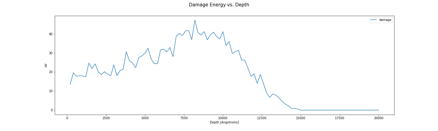
def plot_damage_energy(folder, ax):
results = Results(folder)
phon = results.phonons
dx = max(phon.depth) / 100.0 # to units of Angstroms
energy_damage = (phon.ions + phon.recoils) * dx
ax.plot(phon.depth, energy_damage / phon.num_ions, label='{}'.format(folder))
return sum(energy_damage)
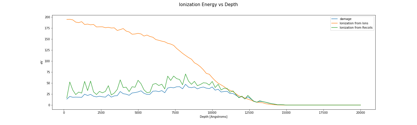
def plot_ionization(folder, ax):
results = Results(folder)
ioniz = results.ioniz
dx = max(ioniz.depth) / 100.0 # to units of Angstroms
ax.plot(ioniz.depth, ioniz.ions, label='Ionization from Ions')
ax.plot(ioniz.depth, ioniz.recoils, label='Ionization from Recoils')
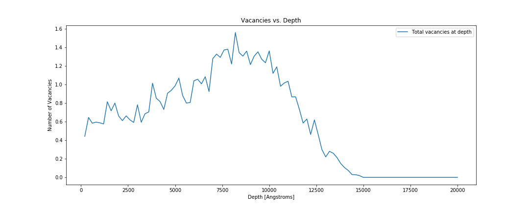
def plot_vacancies(folder, ax):
results = Results(folder)
vac = results.vacancy
vacancy_depth = vac.knock_ons + np.sum(vac.vacancies, axis=1)
ax.plot(vac.depth, vacancy_depth, label="Total vacancies at depth")
return sum(vacancy_depth)
folders = ['test_files/2', 'test_files/4']
image_directory = 'examples/images'
os.makedirs(image_directory, exist_ok=True)
Here we initialize three plotting functions.
Damage energy vs depth.
fig, axes = plt.subplots(1, len(folders), sharex=True, sharey=True)

for ax, folder in zip(np.ravel(axes), folders):
    energy_damage = plot_damage_energy(folder, ax)
    print("Damage energy: {} eV".format(energy_damage))
    ax.set_xlabel('Depth [Angstroms]')
    ax.set_ylabel('eV')
    ax.legend()

fig.suptitle('Damage Energy vs. Depth', fontsize=15)
fig.set_size_inches((20, 6))
fig.savefig(os.path.join(image_directory, 'damagevsdepth.png'), transparent=True)
Ionization energy vs depth
fig, axes = plt.subplots(1, len(folders), sharey=True, sharex=True)

for ax, folder in zip(np.ravel(axes), folders):
    plot_damage_energy(folder, ax)
    plot_ionization(folder, ax)
    ax.legend()
    ax.set_ylabel('eV')
    ax.set_xlabel('Depth [Angstroms]')
fig.suptitle('Ionization Energy vs Depth', fontsize=15)
fig.set_size_inches((20, 6))
fig.savefig(os.path.join(image_directory, 'ionizationvsdepth.png'), transparent=True)
Total number of vacancies vs depth.
fig, ax = plt.subplots()

for i, folder in enumerate(folders):
    total_vacancies = plot_vacancies(folder, ax)
    print("Total number of vacancies {}: {}".format(folder, total_vacancies))

ax.set_xlabel('Depth [Angstroms]')
ax.set_ylabel('Number of Vacancies')
ax.set_title('Vacancies vs. Depth')
ax.legend()
fig.set_size_inches((15, 6))
fig.savefig(os.path.join(image_directory, 'vacanciesvsdepth.png'), transparent=True)
For a much more advanced example please see SiC ion damage production jupyter notebook. This tutorial is also available in notebook form.